

Arithmetic and Geometric Sequences in Python

In mathematics a sequence is an ordered series of numbers called terms, each of which is calculated from the previous using a certain rule. Naturally the number of possible rules is infinite and a rule can become arbitrarily complicated. In this article I will describe and code the two simplest types of rule, arithmetic and geometric.
Arithmetic Sequences
In an arithmetic sequence each term is calculated by adding a fixed number, known as the common difference, to the previous. The first term has to be specified after which as many subsequent terms can be calculated as you need. Note that the common difference can be negative which is equivalent to subtracting a positive number.
There are two ways of evaluating a sequence, applying the rule to the previous value to find the next, or calculating each term individually from its position or index. These are known as the term-to-term rule and the nth term rule respectively.
This is the mathematical notation of the two rules for arithmetic sequences.
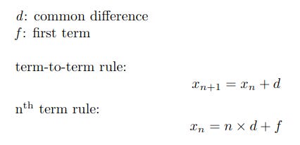
Each term is denoted using xn where n is the index of the particular term. The term-to-term rule simply illustrates the process I described above: add a specified number to the previous term. The nth term rule is slightly more complex but does enable individual terms to be calculated without running through every previous term.
Geometric Sequences
Geometric sequences are very similar to arithmetic sequences but each term is calculated by multiplying each term by a fixed value known as the common ratio. We can also carry out the equivalent of division by multiplying by the reciprocal of the divisor, for example to divide by two just multiply by 1/2.
This is the notation.
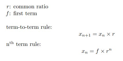
Again the term-to-term rule just mirrors the textual description, and the nth term rule gives us a shortcut to individual terms without calculating all the preceding ones..
The Project
This project consists of the following files:
sequences.py
seqdemo.py
The files can be cloned or downloaded from the GitHub repository.
This article's code uses the NumPy library. If you are not familiar with NumPy you might like to read my article which provides a brief introduction to get you up and running quickly.
The Code
The sequences.py file contains four functions to implement the two methods described above of calculating arithmetic and geometric sequences.
import numpy as np


def arithmetic_ntr(first_value: float = 1,
                   count: int=16,
                   com_diff: float=1):

    """
    Create a sequence where each term is the previous
    term plus a common difference.
    This function uses the n-th term rule to
    calculate each term individually.
    """

    # NumPy array of indexes
    seq = np.arange(0.0, count)

    # calculate values from indexes
    seq = seq * com_diff + first_value

    return seq


def arithmetic_ttotr(first_value: float = 1,
                     count: int=16,
                     com_diff: float=1):

    """
    Create a sequence where each term is the previous
    term plus a common difference.
    This function uses the term to term rule to
    calculate each term from the previous.
    """

    # NumPy array of zeros
    seq = np.zeros(count)

    seq[0] = first_value

    # calculate values from preceding values
    for i in range(1, count):

        seq[i] = seq[i-1] + com_diff

    return seq


def geometric_ntr(first_value: float = 1,
                  count: int=16,
                  com_ratio: float=2):

    """
    Create a sequence where each term is the previous
    term multiplied by a common ratio.
    This function uses the n-th term rule to
    calculate each term individually.
    """

    # NumPy array of indexes
    seq = np.arange(0.0, count)

    # calculate values from indexes
    seq = first_value * (com_ratio**(seq))

    return seq


def geometric_ttotr(first_value: float = 1,
                    count: int=16,
                    com_ratio: float=2):

    """
    Create a sequence where each term is the previous
    term multiplied by a common ratio.
    This function uses the term to term rule to
    calculate each term from the previous.
    """

    # NumPy array of zeros
    seq = np.zeros(count)

    seq[0] = first_value

    # calculate values from preceding values
    for i in range(1, count):

        seq[i] = seq[i-1] * com_ratio

    return seq
arithmetic_ntr
This is the function using the nth term rule, the argument names being self-explanatory, as argument names should be! A NumPy array of zeros is created, and the entire sequence can be calculated in a single line implementing the nth term rule. This is one of the biggest advantages of using NumPy, particularly as this is very fast as we'll see later.
arithmetic_ttotr
This function uses the term-to-term rule and while the sequence is still in a NumPy array the values have to be calculated in a for loop which slows things down considerably.
geometric_ntr
The geometric_ntr function follows the same pattern as arithmetic_ntr but with a slightly different calculation.
geometric_ttotr
Again we have the same pattern as arithmetic_ttotr but with a multiplication.
Demoing the Functions
The seqdemo.py file contains code to run the functions in sequences.py, including timing the two methods, nth term and term-to-term.
import time

import numpy as np

import sequences as seq


def main():

    print("-----------------")
    print("| codedrome.com |")
    print("| Sequences     |")
    print("-----------------\n")

    arithmetic()

    # geometric()

    # arithmetic_timing()

    # geometric_timing()


def arithmetic():

    np.set_printoptions(formatter={'float':lambda x: f"{x:0,.1f}"})

    arithseq = seq.arithmetic_ntr(first_value=3.0, count=24, com_diff=3.0)
    print(arithseq)

    print()

    arithseq = seq.arithmetic_ttotr(first_value=3.0, count=24, com_diff=3.0)
    print(arithseq)


def geometric():

    np.set_printoptions(formatter={'float':lambda x: f"{x:0,.4f}"})

    geomseq = seq.geometric_ntr(first_value=10.0, count=24, com_ratio=1.1)
    print(geomseq)

    print()

    geomseq = seq.geometric_ttotr(first_value=10.0, count=24, com_ratio=1.1)
    print(geomseq)


def arithmetic_timing():

    np.set_printoptions(formatter={'float':lambda x: f"{x:0,.1f}"})

    start = time.perf_counter_ns()
    arithseq = seq.arithmetic_ntr(first_value=3.0, count=10000, com_diff=1.1)
    end = time.perf_counter_ns()
    print(f"n-th term rule {end - start:0,} nanoseconds")

    start = time.perf_counter_ns()
    arithseq = seq.arithmetic_ttotr(first_value=3.0, count=10000, com_diff=1.1)
    end = time.perf_counter_ns()
    print(f"term to term rule {end - start:0,} nanoseconds")


def geometric_timing():

    np.set_printoptions(formatter={'float':lambda x: f"{x:0,.1f}"})

    start = time.perf_counter_ns()
    geomseq = seq.geometric_ntr(first_value=10.0, count=10000, com_ratio=1.001)
    end = time.perf_counter_ns()
    print(f"n-th term rule {end - start:0,} nanoseconds")

    start = time.perf_counter_ns()
    geomseq = seq.geometric_ttotr(first_value=10.0, count=10000, com_ratio=1.001)
    end = time.perf_counter_ns()
    print(f"term to term rule {end - start:0,} nanoseconds")


if __name__ == "__main__":

    main()
arithmetic
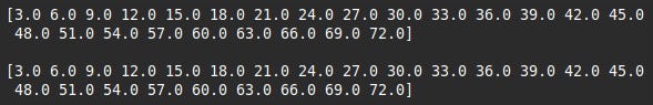
The first line in the arithmetic function tells NumPy to use a custom lambda for formatting output. The function then call the arithmetic_ntr and arithmetic_ttotr, printing the results.
Run the program like this:
python3 seqdemo.py
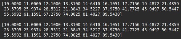
This is the output which you'll be pleased to see is identical for each method of calculation.
geometric
In geometric we do the same thing again, creating and printing sequences using the two methods. Uncomment the function call in main and run the program again.
arithmetic_timing
This function again calls both the arithmetic functions but with a few lines of code to time them. This is done by calling time.perf_counter_ns() before and after the function call and storing the return values (which are in nanoseconds or billionths of a second). Subtracting the first from the second gives us the time taken which is then printed. Uncomment arithmetic_timing and run the program.
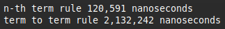
The huge difference in calculating the exact same values in two different ways is due to the nth term rule using pure NumPy vectorized code whereas the term-to-term method uses a Python for loop.
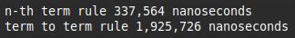
geometric_timing
Lastly we again use the same timing technique but with the geometric functions. The difference is slightly less but still considerable.
No AI was used in the creation of the code, text or images in this article.