

Benford’s Law in Python


In this post I will write a Python implementation of Benford's Law which describes the distribution of the first digits of most sets of numeric data.
I recently posted an article on Zipf's Law and the application of the Zipfian Distribution to word frequencies in a piece of text. Benford's Law can be considered a special case of Zipf’s Law.
Applying the Zipfian Distribution to bodies of text is fraught with difficulty due to the vagaries of natural language and I am sceptical of the practicalities and usefulness of doing so beyond demoing the Zipfian Distribution and its implementation.
However, the Benford Distribution is very different. If you have a set of numeric data you can try to fit it to the Benford Distribution without worrying about all the quirks and messiness of natural language. You don't even have to worry about the total number of possible distinct values - every number starts with 1 to 9.
Benford's Law centres on the perhaps surprising fact that in numeric data such as financial transaction, populations, sizes of geographical features etc. the frequencies of first digits follow a roughly reciprocal pattern. This is shown in the following table, the relative frequencies being calculated using the formula in the heading of the right hand column.
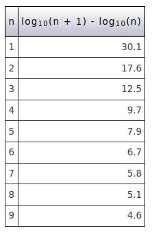
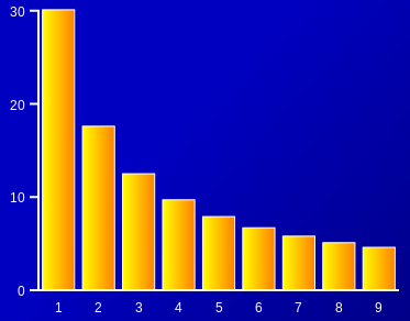
If the first digits followed a uniform distribution which you might intuitively expect each digit would appear about 11% of the time. However, in the Benford Distribution the number 1 occurs about 30% of the time, 2 about 18% of the time etc.. This is clearer when shown in a graph.
The best known use of Benford's Law is in fraud detection. If someone makes up false data it is unlikely to follow the Benford Distribution you would expect from genuine data, and if the numbers are purely random the first digits would probably fit a uniform distribution, ie. 11% each as described above.
* I have mentioned first digits several times and you may be wondering about subsequent digits. Do they also fit the Benford Distribution? The answer is yes but to a decreasing amount. As you move along the digits the distributions become less Benfordian and more uniform.
For this post I'll write a function to take a list of numbers and create a table of values showing how closely it fits the Benford Distribution.
I'll then try it out with two sets of data, a fraudulent-looking one which roughly fits the uniform distribution and a genuine-looking one which roughly fits the Benford Distribution. I will also create a simple console graph to show the results.
The project consists of two files:
benfordslaw.py
benfordslaw_demo.py
The files can be cloned or downloaded from the Github repository.
This is the first file, benfordslaw.py.
benfordslaw.py
import collections


BENFORD_PERCENTAGES = [0, 0.301, 0.176, 0.125, 0.097, 0.079, 0.067, 0.058, 0.051, 0.046]

def calculate(data):

    """
    Calculates a set of values from the numeric list
    input data showing how closely the first digits
    fit the Benford Distribution.
    Results are returned as a list of dictionaries.
    """

    results = []

    first_digits = list(map(lambda n: str(n)[0], data))
    first_digit_frequencies = collections.Counter(first_digits)

    for n in range(1, 10):

        data_frequency = first_digit_frequencies[str(n)]
        data_frequency_percent = data_frequency / len(data)
        benford_frequency = len(data) * BENFORD_PERCENTAGES[n]
        benford_frequency_percent = BENFORD_PERCENTAGES[n]
        difference_frequency = data_frequency - benford_frequency
        difference_frequency_percent = data_frequency_percent - benford_frequency_percent

        results.append({"n": n,
                        "data_frequency":               data_frequency,
                        "data_frequency_percent":       data_frequency_percent,
                        "benford_frequency":            benford_frequency,
                        "benford_frequency_percent":    benford_frequency_percent,
                        "difference_frequency":         difference_frequency,
                        "difference_frequency_percent": difference_frequency_percent})

    return results
Firstly we import collections to use collections.Counter. Then comes a constant list of the relative frequencies of the digits 1 to 9 as decimal fractions. I have padded it out with a superfluous 0 so we can index the values using the digits they represent. It is up the top outside the function so it can be used by external code.
The calculate function takes a list and creates from it a list of the first digits (as strings) which is then used to construct a collections.Counter. This object now contains a set of key/value pairs for each distinct first digit. A useful feature of Counter is that if we try to access a key which does not exist it will return 0.
Next we need to iterate from 1 to 9, calculating a few values for each digit showing how it compares to the Benford Distribution. These are then used to create dictionaries which are added to a list which is then returned.
Now we can try the module out in benfordslaw_demo.py.
benfordslaw_demo.py
import random

import benfordslaw


def main():

    print("-----------------")
    print("| codedrome.com |")
    print("| Benford's Law |")
    print("-----------------\n")

    data = get_random_data()
    #data = get_benford_data()

    print(len(data))

    benford_table = benfordslaw.calculate(data)
    print_as_table(benford_table)
    print()
    print_as_graph(benford_table)


def get_random_data():

    """
    Returns a list of 1000 numbers approximately
    following the uniform distribution NOT the
    Benford Distribution.
    """

    random_data = [0] * 1000

    random_data = list(map(lambda n: n + random.randint(1, 1000), random_data))

    return random_data


def get_benford_data():

    """
    Returns a list of about 1000 numbers
    approximately following the Benford Distribution.
    """

    benford_data = []

    for first_digit in range(1, 10):
        random_factor = random.uniform(0.8, 1.2)
        for num_count in range(1, int(1000 * benfordslaw.BENFORD_PERCENTAGES[first_digit] * random_factor)):
            start = first_digit * 1000
            benford_data.append(random.randint(start, start + 1000))

    return benford_data


def print_as_table(benford_table):

    width = 59

    print("-" * width)
    print("|   |      Data       |    Benford      |    Difference   |")
    print("| n |  Freq     Pct   |  Freq     Pct   |  Freq     Pct   |")
    print("-" * width)

    for item in benford_table:

        print("| {} | {:6.0f} | {:6.2f} | {:6.0f} | {:6.2f} | {:6.0f} | {:6.2f} |".format(item["n"],
                                   item["data_frequency"],
                                   item["data_frequency_percent"] * 100,
                                   item["benford_frequency"],
                                   item["benford_frequency_percent"] * 100,
                                   item["difference_frequency"],
                                   item["difference_frequency_percent"] * 100))

    print("-" * width)


def print_as_graph(benford_table):

    REDBG = "\x1B[41m"
    GREENBG = "\x1B[42m"
    RESET = "\x1B[0m"

    print("  0%       10%       20%       30%       40%       50%       60%       70%       80%       90%       100%")
    print("  |         |         |         |         |         |         |         |         |         |         |\n")

    for item in benford_table:

        print(" {} {}\n   {}\n  ".format(str(item["n"]),
                                         GREENBG + (" " * int(round(item["benford_frequency_percent"] * 100))) + RESET,
                                         REDBG + (" " * int(round(item["data_frequency_percent"] * 100))) + RESET))


main()
main
After importing random and benfordslaw we enter the main function. This calls one of two functions to get some test data, and then throws it at benfordslaw.calculate. The results are then passed to print_as_table and print_as_graph.
get_random_data
This is a simple function which creates 1000 random values between 1 and 1000.
get_benford_data
This is more complex because it creates about 1000 values which roughly fit the Benford Distribution. For each digit 1-9 it iterates from 1 to the proportion of each digit in the Benford Distribution, retrieved from the benfordslaw module. So we don't get an exact fit each time this is adjusted by a random amount between 0.8 and 1.2. Within this loop we create a set of values with the relevant first digit.
print_as_table
A fiddly but straightforward function to print out the data structure returned by benfordslaw.calculate in a table.
print_as_graph
This also takes the data structure returned by benfordslaw.calculate and prints it as a graph in the console. Firstly we define some ANSI terminal colour constants and after some hard-coded headings we iterate the data, printing out the Benford and actual frequencies as bars in green and red respectively.
That's the coding finished so let's run the program.
python3.7 benfordslaw_demo.py
This is the output with random data.

The green Benford Distribution bars are always the same but the red bars show the actual distribution. In this case we can easily see that the actual distribution is roughly uniform and doesn't fit the Benford Distribution at all. Very suspicious!
In main comment out data = get_random_data(), uncomment data = get_benford_data() and run the program again.

This set of data is a much better fit to Benford's Distribution. If we didn't know better we would think it was genuine!