

First Steps in Isometrics with Python

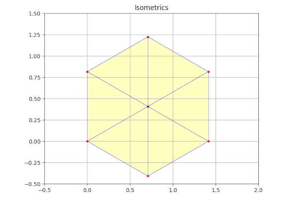
The word isometric means “with equal measurements” and the best known use of the word is probably as a form of “pseudo-3d” graphics without perspective. This means that a particular distance will appear on screen the same size irrespective of its supposed distance from the viewer. You may already be familiar with isometric projections even if you didn’t know the term as they have been used for decades in video games, and are far simpler to calculate than true 3d coordinates.
In this article I’ll write a very minimalist introduction to the subject which will calculate the two-dimensional coordinates of a three-dimensional cube, and then plot them using Matplotlib. As the title of the article states this is very much a first step and I have a number of ideas for taking isometrics further.
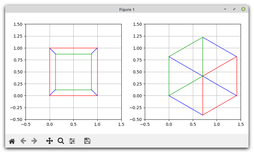
The screenshot below illustrates just what we are going to achieve. The cube on the left is shown with perspective, the red lines being the near face and the green lines being the far face. On the right is the same cube but with the vertices (corners) and edges (lines between corners) calculated to give an isometric projection. The colours remain the same so you can see how the cube has been rotated right and down, although it’s probably better to think of the viewer moving left and up.
The process of calculating the data we need to plot the cube on the right consists of the following steps:
Create a set of 8 three-dimensional coordinates for the corners or vertices of the cube. These each consist of 3 values: x (horizontal), y (vertical) and z (front to back)
For each vertex calculate the two-dimensional x and y values. This is the core calculation for the whole field of isometrics.
From the 2d vertex coordinates create edges consisting of two coordinates each.
Also using the 2d vertex coordinates, calculate the top, bottom, left and right borders of the three visible faces of the cube.
Having carried out the following steps we can pass the data to Matplotlib so it can do its thing and produce output like that shown above.
The Dreaded Mathematics (Optional)
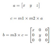
Calculating two-dimensional x,y coordinates from three-dimensional x,y,z coordinates is an involved process using matrices, some of the matrices used having their values calculated using trigonometric functions. Untangling the trigonometry and matrix arithmetic is way beyond the scope of a programming article although I may write about it on my LaTeX Substack.
I’ll therefore just give a very brief overview of the process to give a flavour of what is going on. Don’t worry if you don’t understand this, and please feel free to skip to the next section if you aren’t interested in the mathematics.
There are three broad stages involved.
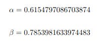
Create Constants α and β
These two constants are angles in radians.
Create Three Matrices
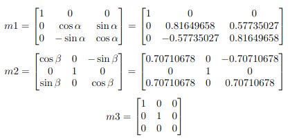
These are effectively constant although many of the values are calculated using α, β and trigonometry.
Calculate Two-Dimensional Coordinates
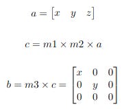
The first matrix, a, contains the three-dimensional coordinates. The second, c, is the product of m1 and m2 from the second stage and a.
Finally, m3 and c are multiplied to create a matrix containing the x and y coordinates. (The others are always 0 and superfluous.)
The Project (Back to Python!)
This project consists of the following files which you can clone or download from the Github repository.
isometric.py
isometricplotter.py
isometricdemo.py
isometricillustrator.py
The last of these, isometricillustrator.py, creates the side-by-side plots shown above. I won’t show the code here as it’s basically just a load of hardcoded coordinates.
The code uses NumPy and Matplotlib. If you are not familiar with these please read my introductory articles on them.
https://codedrome.substack.com/p/a-numpy-reference
https://codedrome.substack.com/p/a-matplotlib-reference
isometric.py
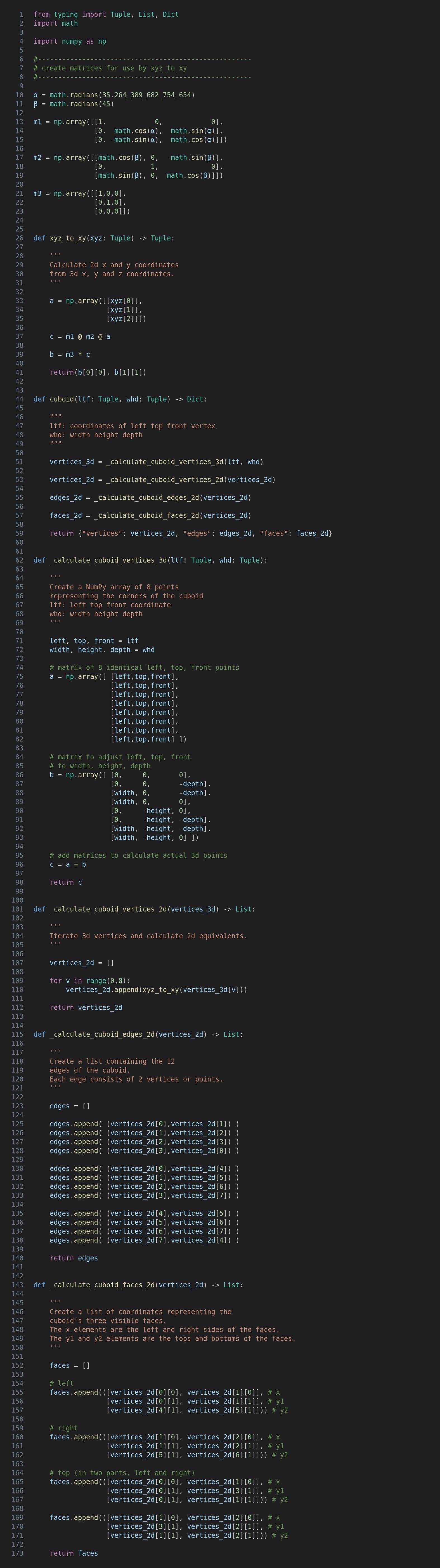
This is the code for isometric.py which implements the mathematics shown above, and also calculates the vertices, edges and faces of a cuboid.
Constant Values and Matrices
These are the constants which form the first step of the calculations. The symbols are the Greek letters alpha and beta and although I rarely use characters in code that aren’t on my keyboard I decided to do so here to conform to the usual conventions for these calculations.
The matrices m1, m2 and m3 are then created, partly using sine functions and α and β, and partly hard-coded.
xyz_to_xy
This function is at the heart isometric rendering as it converts three-dimensional coordinates to two dimensions, specifically x,y,z to x,y. If you wish to follow the mathematics the code corresponds to the following, repeated from above.
cuboid
This function creates a dictionary of vertices, edges and faces which make up a cuboid with the specified position and size. The separate elements are generated by the various functions described below.
_calculate_cuboid_vertices_3d
This function’s parameters are the ltf (left, top, front) and whd (width, height, depth) arguments from the cuboid function, split out into separate variables to make them easier to use.
Firstly a NumPy array is created to represent a matrix with all values the same, specifically the left top front vertex. The second array contains values specifying how much each point has to be shifted in each axis. By adding these together we end up with a matrix of coordinates of the eight vertices.
_calculate_cuboid_vertices_2d
This function “flattens” the 3D coordinates down to 2D by calling xyz_to_xy on each one and adding the result to a list.
_calculate_cuboid_edges_2d
The twelve edges are created rather tediously by appending the necessary pairs of vertices to a list. I couldn’t discern a pattern to the indices that could be used to streamline the process - if you can then please let me know or, better still, write a shorter and neater version of this function. Thank you.
_calculate_cuboid_faces_2d
Here we create a list of the coordinates of the vertices of the front faces of the cuboid, the ones that can be seen and need filling. The same comment applies as with _calculate_cuboid_edges_2d: if you can make it more concise please do so.
isometricplotter.py
The isometricplotter.py file contains code to plot isometric objects.
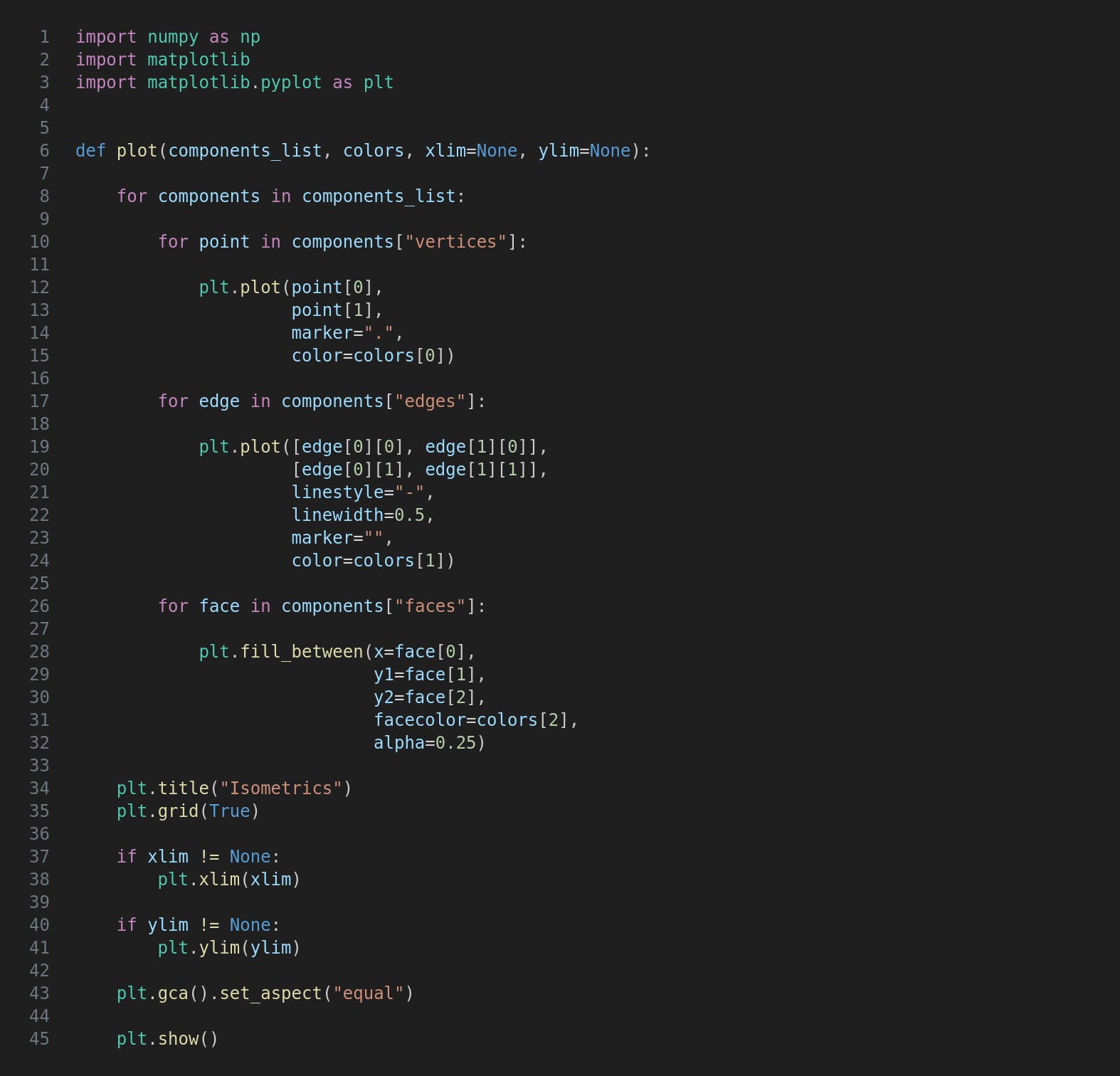
The components list is iterated with a for/in loop which in turn iterates and plots the three types of element making up each shape. The vertices are plotted first; note the marker is set to “.” and that the first colour in the list is used. The edges have no markers, a linestyle of “-” and are drawn with the second colour.
Finally the faces are drawn with the fill_between method which, to quote the documentation, “fills the area between two horizontal curves”. Each coordinate argument, x, y1 and y2, consists of two coordinates so together they make up a two-dimensional area to fill. The last of the colours is used, and I have set alpha or opacity to 0.25 so the bits of the cuboid hidden by faces are still visible.
isometricdemo.py
In isometricdemo.py we try out the code listed above.
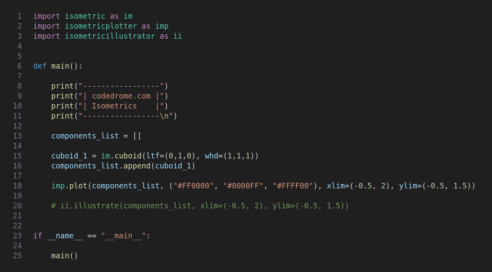
The isometricplotter’s plot function takes a list of components to plot so first we create an empty list, then create a single cuboid which is appended to the list. Finally this list is passed to plot along with a few other arguments as described above.
The commented line calls a function to create the double plot showing a colour-coded illustration of the rotation process.
Running the Program
Run the program like this:
python3 isometricdemo.py
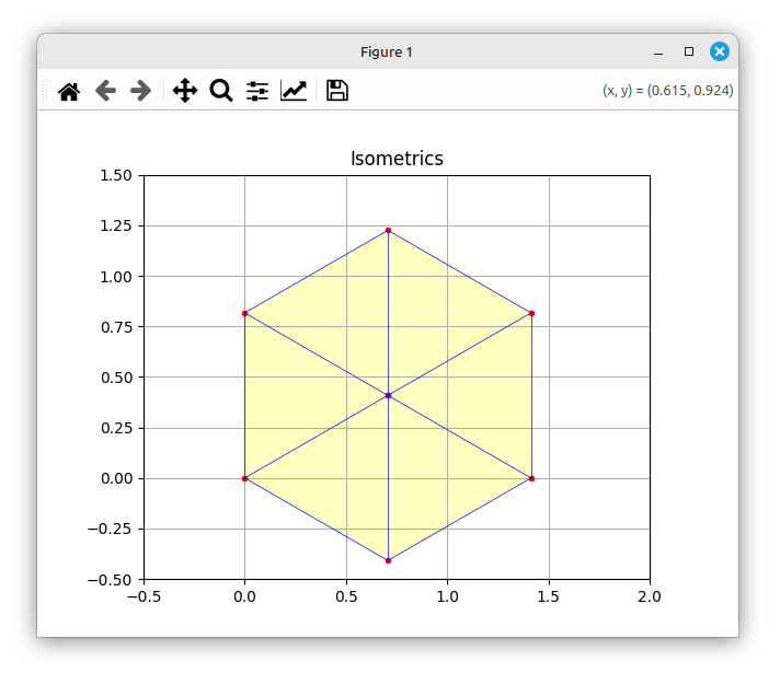
This is the end result.
Conclusion
The code which calculates two-dimensional coordinates from three-dimensional ones is at the core of isometrics so by coding this process we have laid a firm foundation, as well as put it to good use by drawing a “box”. However, this is only the first step and in future articles I will use the code in PyGame and add further shapes.
For updates and random ramblings please follow me on Bluesky.
No AI was used in creating the code, text or images in this article.