

Quadratic Functions in Python part 1: Areas of Squares


The word quadratic derives from the Latin quadratus meaning square and in its simplest form a quadratic function calculates the areas of squares from the length of a side. In this article, the first of a series, I will write Python code to calculate and areas of squares and graph them using the Matplotlib library.
The quadratic equation looks like this:
and is a statement of fact rather than a description of how to calculate the areas of squares or any real-world objects or behaviour. Specifically, it states that for a maximum of two values of x the equation evaluates to 0. Calculating these values of x will be the subject of a future article.
To calculate values of y, for example the areas of squares, for a range of values of x or lengths of a side we need the equation in the form of a function like this.
The letters a, b and c are called coefficients and are constant for a given specific function irrespective of the values of x. Again I'll describe and code the usage of coefficients in a future article but for this article, calculating the areas of squares, we just need the simplest possible quadratic function:

This tells us what everyone knows already: to work out the area of a square multiply the length of a side by itself, or in other words square it. The values of x can be any real number including 0 or negative. This is more formally known as the domain of the function and I'll go into this topic in more detail in the future along with the related topic of the function's domain or possible values of y. For now I'll stick with values of x which are >= 0 to represent actual squares.
The Project
This project consists of the following files:
qf1.py
qfdemo1.py
which you can clone or download from the GitHub repository
The code for this article uses the NumPy and Matplotlib libraries. If you are not familiar with these you might like to read my reference articles on them to get you up 'n' running quickly.
The Code
The first file, qf1.py, contains a class with properties representing the coefficients as well as methods to evaluate the function for specified values of x, print the x and y values and graph them. (Having three areas of functionality, calculation, printing and graphing in one class is not good practice and if this project grows significantly I'll separate them.)
from typing import Tuple

import numpy as np
import matplotlib
import matplotlib.pyplot as plt


matplotlib.use('Qt5Agg')


class QuadraticFunction(object):

    '''
    The QuadraticFunction class has properties
    representing the coefficients of a function
    in the general form.
    The class has methods to evaluate the function for
    given x values, and print and plot x and y.
    '''

    def __init__(self,
                 a: float=1,
                 b: float=0,
                 c: float=0):

        self.a = a # quadratic coefficient
        self.b = b # linear coefficient
        self.c = c # constant coefficient

        self.equation_str = self.__create_eq_str()

        self.xvalues = None
        self.yvalues = None


    def evaluate(self, xminmax: Tuple=(-10.0,11.0), interval: float=1.0) -> None:

        '''
        Populates the instance's xvalues and yvalues
        using coefficient properties.
        Arguments:
            xminmax - tuple of min and max x values
            interval - between x values
        Return:
            none
        '''

        # create a lambda based on x and coefficients
        func = lambda x: self.a*x**2 + self.b*x + self.c

        self.xvalues = np.arange(xminmax[0], xminmax[1], interval)

        self.yvalues = func(self.xvalues)


    def print_values(self) -> None:

        '''
        Prints intance's xvalues and yvalues in a table format.
        '''

        heading = "       x           y  "

        print("-" * len(heading))
        print(heading)
        print("-" * len(heading))

        for i in range(0, len(self.xvalues)):

            print(f"{self.xvalues[i]:>9.2f}", end="")
            print(f"{self.yvalues[i]:>13.2f}")

        print("-" * len(heading))


    def plot(self, color: str='#FF4000') -> None:

        '''
        Plot the xvalues and yvalues using specified color.
        '''

        plt.plot(self.xvalues,
                 self.yvalues,
                 color=color)

        plt.xlabel("x")
        plt.ylabel("y")
        plt.title(f"{self.equation_str}")
        plt.grid(True)

        plt.show()


    def __create_eq_str(self) -> str:

        return f"y = {self.a}x² + {self.b}x + {self.c}"
__init__
The three parameters are for the three coefficients mentioned above. The defaults have no effect on the values of y as they multiply the result of the squaring by 1, add 0 and then add 0 again, the result being no change.
The equation_str property is set with the __create_eq_str which I'll describe later, and finally a pair of properties for the x and y values are created and initialised to None. They will be given proper values by the evaluate method.
evaluate
The evaluate function takes as arguments minimum and maximum values of x as well as an interval between consecutive values. It then sets the class's xvalues using these arguments and finally calculates the y values for each x value.
The quadratic function itself is created as a lambda using the coefficient properties. The lambda is then used in the last line - as we are using NumPy the iteration is abstracted away and the function can be called on the entire array in one go.
print_values
Firstly a heading for x and y values is printed with lines made up of the - character, followed by a for loop to iterate and print the values.
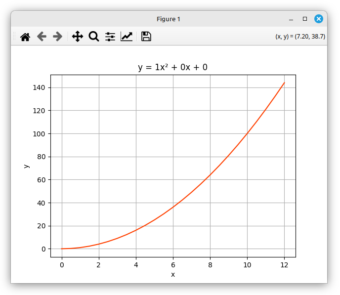
plot
This is a very simple usage of Matplotlib and all we are doing is throwing the xvalues and yvalues properties at the plot method. The color argument isn't strictly necessary of course but you might consider orange to be more interesting than the default blue. The next four lines are cosmetic but pretty necessary for the plot to make sense; note that the title is set to the human-readable string created by the following function.
__create_eq_str
This is a "pseudo-private" function (as denoted by the double underscores) which arranges the coefficients into a string representation of the function for the calling code to use for any form of user output that may be needed.
Now we can move on to a a short bit of code to demo the QuadraticFunction class
import qf1
def main():
print("-------------------------")
print("| codedrome.com |")
print("| Quadratic Functions 1 |")
print("-------------------------\n")
qf = qf1.QuadraticFunction()
qf.evaluate(xminmax=(0.0, 12.1), interval=0.5)
print(f"{qf.equation_str}\n")
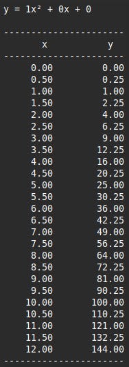
qf.print_values()
qf.plot()
if __name__ == "__main__":
main() After importing qf1 the main function creates a QuadraticFunction object; there are no arguments so the defaults are used. The evaluate method is given a range of non-negative values representing actual box sides. Then we just print the equation_str property and call the print_values and plot methods.
Running the Program
That's the coding done so run the program with this command:
python3 qfdemo1.py
This is the terminal and Matplotlib output.
As well as calculating the areas of squares quadratic functions can be used to model a vast range of real world phenomena. Most of those won't fit neatly into a basic unmodified function such as that shown here and it will be necessary to stretch, squash and move the graph around. These tasks, more properly known as transforms and translations, are accomplished by using coefficient values other than the defaults set in __init__ and this topic will be covered in the next article.
No AI was used in the creation of the code, text or images in this article.