

Quadratic Functions in Python part 3: Solving Equations


Overview
This is Part 3 of my series on quadratic functions. These are the first two:
Quadratic Functions in Python part 1: Areas of Squares
Quadratic Functions in Python part 2: Coefficients
The articles linked above covered quadratic functions of the form...
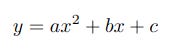
...which are used to calculate and plot a series of y values from x values using coefficients a, b and c.
In this article I’ll demonstrate how to solve the following equation.
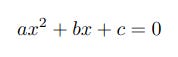
which basically describes a special case of the quadratic function for which y = 0. Solving the equation involves using given values of the coefficients a, b and c to find what are termed the roots of the function, ie the two values of x for which the equation holds true; in practical terms this means finding the values of x where the curve crosses the x-axis.
There are three main ways of accomplishing this, two of which are factoring and completing the square. If you have to carry out the task by hand with no more than a pencil and piece of paper then these are probably easier but they are fiddly to code and I really don’t see the point of attempting to do so. I will therefore be using the third method, the quadratic formula which is shown below.
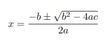
This method clearly isn’t pencil-and-paper friendly but it’s easy to code and in fact you don’t even have to do that - I’ve done it for you! (I’d encourage you to try anyway.) Note that the equation includes the plus and minus symbol ± which means it is two calculations in one, the first using addition and the second using subtraction. The two results are the roots of the equation for a specific set of coefficients.
As we’ll see shortly, for certain combinations of coefficients the curve’s vertex (highest or lowest point) touches the x-axis at just one point in which case the equation is said to have one repeated root.
Other combinations of coefficients can result in the curve not intercepting the x-axis at all. In these cases the roots still exist but are complex* numbers. The whole field of complex numbers is huge and, well, complex and way beyond a simple little article like this. The code below will show complex results for completeness but unless you are already familiar with the field just interpret these as meaning the curve doesn’t intercept the x-axis.
* Strictly speaking all numbers are complex but it isn’t usual to include the imaginary bit if it’s 0. Writing “2.0 + 0i bottles of milk” on your shopping list is a bit tedious.
The Project
This project consists of the following files:
qf2.py
qfplotter.py
qfdemo3.py
which you can clone or download from the GitHub repository The depository will be used for all files for this series of articles.
The code for this article uses the NumPy and Matplotlib libraries. If you are not familiar with these you might like to read my reference articles on them to get you up ‘n’ running quickly.
The QuadraticFunction Class
The QuadraticFunction class in qf1.py has been expanded from the first two articles so I’ll just show the new and modified functions in qf2.py.
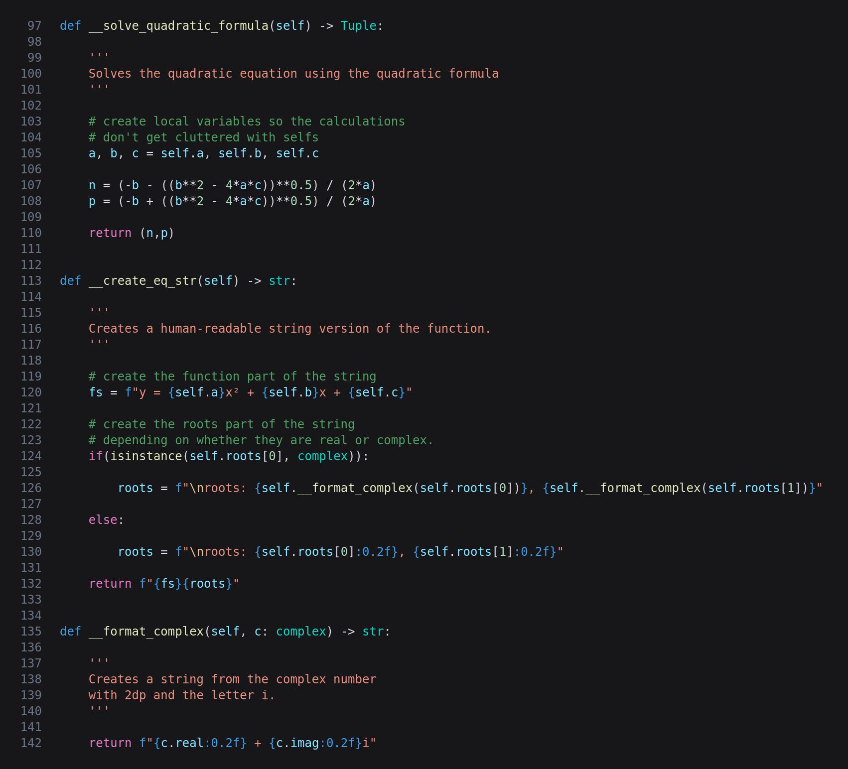
__solve_quadratic_formula
This function is called in __init__ so does not need to be called separately by the code creating instances of the QuadraticFunction class. The coefficients are used five times in each of the two variations of the formula so I have copied the properties to local variables so there aren’t loads of selfs scattered around.
Next we have two nearly identical lines of code, the only difference being the minus in the first and plus in the second. I tried to think of ways to streamline this but they would have been more complicated than just having two near repetitions so I decided to go with that. If you know of a neat, elegant and compact way of merging the calculations then please let me know.
It is important to note here that if there are no real roots Python will automatically give us a complex number.
Finally the two roots are returned as a tuple.
__create_eq_str
This has been expanded to include the roots. The function itself is assembled into the fs variable from the coefficient properties, after which the roots variable is set depending on whether they are real or complex. I have shifted the formatting of complex numbers into strings off to a separate function. Both real and imaginary numbers are trimmed to 2 decimal places.
The return value is the concatenation of fs and roots.
__format_complex
This takes a complex number and formats it to something like 0.00 + 8.49i. Python can create its own strings from complex numbers but I don’t like the results so created my own.
The qfplotter Module
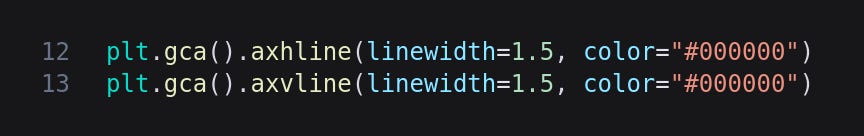
The only change to qfplotter.py from the previous article is a couple of lines to make the x and y axes a bit thicker so the plots are easier to interpret.
qfdemo3.py
The following is used to demonstrate the additions to the code described above.
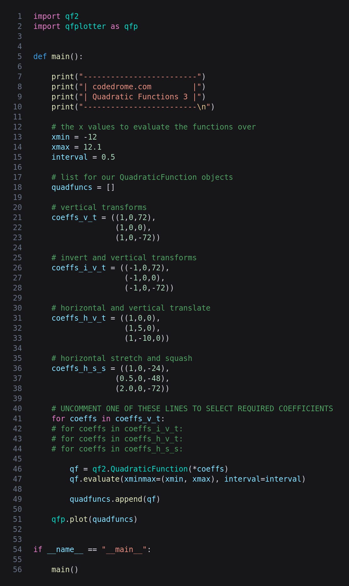
In main we have four tuples-of-tuples containing coefficients to try out the root-finding code. They create selections of translations and transformations, and the cryptic abbreviations are explained in the comments. You can of course change these or add your own using any combination of a, b or c subject to the restriction that a cannot be 0. That would cause the dreaded divide by zero error in the quadratic formula so I must remember to add validation to a later version.
Near the end of main the tuples are iterated in a for-in loop and used to create QuadraticFunction objects which are appended to a list. Remember that in each instance __solve_quadratic_formula is called to set the roots property. Finally the list is passed to qfplotter’s plot method.
Running the Program
That’s the coding done so run the program with this command:
python3 qfdemo3.py
This is the plot from the first set of coefficients, coeffs_v_t.
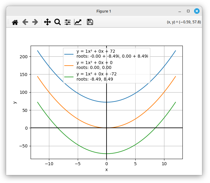
The top blue curve is entirely above the x-axis so the roots are complex numbers. The vertex of the orange curve touches the x-axis so we have a repeated root, and the green curve intersects in two places, -8.49 and 8.49.
If you uncomment the coeffs_i_v_t line and re-run the code you’ll see this plot.
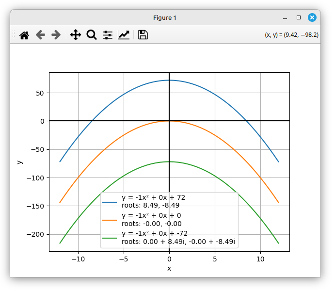
This is similar to the previous sets of coefficients, one curve having two distinct roots, one having a repeated root, and one having complex roots as it doesn’t intersect with the x-axis.
Now let’s try the coeffs_h_v_t coefficients.
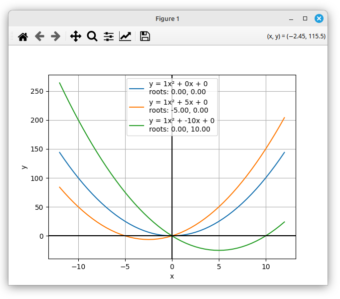
All three intersect the x-axis so there are no complex roots, but the real roots are a bit more interesting as a result of the b coefficient shifting the parabola both horizontally and vertically as described in Part 2.
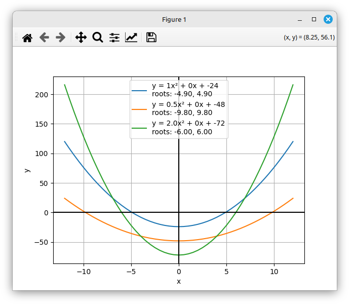
The last sets of coefficients are coeffs_h_s_s which have both a and c changed from the defaults.
I have now covered the basics of evaluating and plotting quadratic functions and also solving quadratic equations, and have written code to do just that with any possible coefficients you can think of. This is, however, a vast topic and I have a number of other articles coming up in which I’ll take things to a more advanced level.
No AI was used in the creation of the code, text or images in this article.